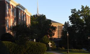
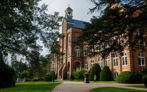
Welcome to the Hilltop
Since 1889, Saint Anselm College has provided a transformative education shaped by Catholic and Benedictine values and a liberal arts foundation. Here, you are part of a welcoming community where you will discover your passions, experience cherished traditions, and unlock your full potential.
Top100.00100
national liberal arts college by Forbes
99.0099%
of identified graduates of the class of 2023 are either employed, pursuing further education, serving in the military, or volunteering
#24.0024
most engaged in community service by Princeton Review
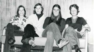
Celebrating 50 Years of Women’s Education
This year marks 50 years of women’s education and achievements at Saint Anselm College. To commemorate this extraordinary milestone, the college is celebrating with events and programs centered around the women of the past and present who have made Saint Anselm College what it is today.
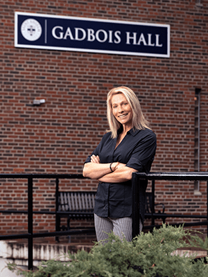
Meet Our Anselmians

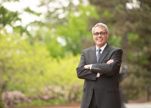
"I believe with all my heart that today’s world needs Saint Anselm College, a place that is infused with the Catholic and Benedictine values of community, hospitality and love, where the humanities, arts and sciences and professional programs like nursing, criminal justice and business build on our liberal arts core rather than compete with it. We need a place where you don’t have to choose between career outcomes and life outcomes. That place is Saint Anselm."
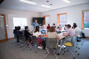
In the classroom and in the community, an Anselmian education will challenge you to find your best self.
Anselmian News
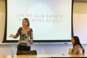
Interdisciplinary Special Topics Course is “Unlike Any Other”
Last fall, a new special topics course blended history and literature in a…
Anselmians Make Record Gifts to Support Saint Anselm College Now and Always
During the 10th annual Days of Giving campaign, the college a record $1.43…
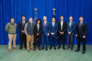
Saint Anselm students play role in President Biden’s NH visit
Students reflect on the important role they played in President Biden’s…

Chapel Arts Center Hosts a Retrospective on long-time Photography Professor
“The Intimacy of Seeing: Elsa Voelcker – A Retrospective,” the current…

Meelia Center's 32nd Annual Valentine's Dance Spreads Love and Inclusion in the Community
The Meelia Center for Community Engagement spread love in the community as…
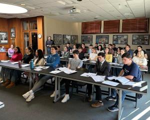
NHIOP Welcomes 2024 Cohort of Kevin B. Harrington Student Ambassadors
The New Hampshire Institute of Politics welcomes 29 new Student Ambassadors…
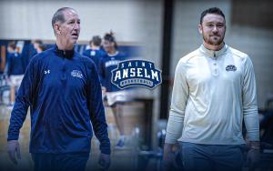
Saint Anselm Men’s Basketball Coach Keith Dickson Announces Retirement; Chris Santo ‘15 Named New Head Coach
After 38 years and 719 victories across 37 seasons, Saint Anselm College…
Write-In | April 16 | 7-10 p.m.
Get your writing done in the company of others!
The Academic…
FEATURED FACULTY MEMBER
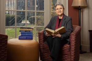
Theology Professor Ahida Pilarski, Ph.D. was featured in the most recent issue of Portraits Magazine's Focus on Faculty.
"The first program in women’s studies in the United States was approved at San Diego State University in 1970. Saint Anselm College also is celebrating the 50th anniversary of women at the college this year. It is nice to know that our college joined this major change of increasing the access of women to education."
Anselmian Events

On Thursday, April 18, 2024 at 9:30 a.m., we will be meeting in the Library Classroom (upper level of Geisel) to discuss "Mexican Gothic" by Silvia Moreno-Garcia.
Description
"After receiving a frantic letter from her newly-wed cousin begging for someone to save her from a mysterious doom, Noemí Taboada heads to High Place, a distant house in the Mexican countryside. She’s not sure what she will find...[and] mesmerized by the terrifying yet seductive world of High Place, may soon find it impossible to ever leave this enigmatic house behind" (GoodReads.com).
All are welcome to attend.
Learn more about our book group by visiting our group webpage.
The Respect the Nest Committee and the Green Team are hosting Saint Anselm College’s first annual Earth Day Fair on Thursday, April 18th. The Fair will take place on JOA Quad/Campus Green and will feature 25+ different clubs, organizations, and academic departments all discussing how environmental initiatives and sustainability relate to and benefit their missions. The present organizations will be tabling with interactive activities for community members to participate in. There will also be free merch, various giveaways, and a plant based BBQ by AVI Dining Services.
The New Hampshire Institute of Politics, in partnership with the Center for Ethics in Society and the Honors Program, is pleased to welcome Morgan Marietta as part of our spring Speaker Series.
About the speaker: Morgan Marietta is Dean of the Center for Economics, Politics & History at the University of Austin. Prior to joining the University of Austin, he taught at the University of Massachusetts Lowell for eleven years and served as Chair of Political Science (briefly) at the University of Texas at Arlington. He studies the political consequences of belief, focusing on constitutional politics, political psychology, and facts in politics.
Marietta is the author of four books, including A Citizen’s Guide to American Ideology, A Citizen’s Guide to the Constitution and the Supreme Court, The Politics of Sacred Rhetoric: Absolutist Appeals and Political Persuasion, and most recently One Nation, Two Realities: Dueling Facts in American Democracy.
His studies of contemporary politics, including absolutist rhetoric, ideological premises, the rhetoric of reality, and the role of hubris have appeared in the leading journals in political science, including the Journal of Politics, British Journal of Political Science, and the American Political Science Review. He is the founding editor of the annual SCOTUS series at Palgrave Macmillan on the major rulings of the Supreme Court, now in its sixth year, and is a regular commentator on the Court at TheConversation.com. His current book project is The Supreme Court of Facts, on the role of the Court in settling disputed perceptions of reality.
In partnership with the Center for Ethics in Society and the Honors Program at Saint Anselm College.
Free and open to the public.
Visit www.anselm.edu/nhiop for the latest news and event information.
Event details for Facts in Politics and the Problem of Hubris
HOPE is a faith-based group that meets once a week. All people are welcome, regardless of where you are on your faith journey. While we will be reading from the Christian Bible and discussing Jesus and the Christian faith, please note that anybody of any faith is welcome to come, hear others, and share their heart.
Contact us for more info: Campusministry@anselm.edu

Join housing experts from The Pew Charitable Trusts to discuss their latest research on policy changes that are improving housing supply and affordability.
The discussion will examine how policymakers across the country are effectively addressing housing shortages, soaring costs, and limited access to financing. In particular, the event will cover multiple topics at the heart of current housing policy debates, including rents and effects on housing costs, public opinion, homelessness, parking, accessory dwelling units and manufactured housing.
Event details for How are policymakers improving access to lower-cost homes?
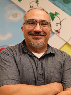
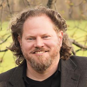
What makes a college Catholic?
Dr. Duane Bruce